Simple walkthrough#
The heart of the DDM code (found in the ddm_calc.py file) is the computation of the image structure function. This is found by taking the average of the Fourier transforms of all image differences. By “image differences,” I mean the result of subtracting two images separated by a given lag time \(\Delta t\).
To describe the process mathematically, we find the difference between images separated by some lag time \(\Delta t\):
For a given \(\Delta t\) all such image differences are calculated. We then Fourier transform each \(\Delta I\) and average all of the same \(\Delta t\).
This results in the image structure function \(D(q_x,q_y,\Delta t)\).
Importing the necessary modules#
Modules for plotting#
We use matplotlib for creating figures and plots. Note that we use:
%matplotlib inline
This sets the backend of matplotlib to inline which means the plots are included in the notebook. If you want the plots to also be interactive (e.g., having the ability to zoom, scroll, and save) then use:
%matplotlib notebook
[1]:
%matplotlib inline
import matplotlib
import matplotlib.pyplot as plt
Modules for numerical work#
Here, we import numpy and xarray.
Note that xarray might not have come with your Anaconda Python distribution (or whichever other distribution you installed). If that is the case, you’ll need to install this package.
[2]:
import numpy as np #numerical python used for working with arrays, mathematical operations
import xarray as xr #package for labeling and adding metadata to multi-dimensional arrays
Import the PyDDM package#
Make sure you append to sys.path the directory containing the PyDDM code.
[3]:
import sys
sys.path.append("../../PyDDM") #must point to the PyDDM folder
import ddm_analysis_and_fitting as ddm
Initializing DDM_Analysis class and computing the DDM matrix#
The instance of the DDM_Analysis class we create will need, when initialized, metadata about the images to analyze and the analysis and fitting parameters. This can be done by using a yaml file as shown in the following cell of code (there, the metadata is saved in the file “example_data_silica_beads.yml”. But one can also initialize DDM_Analysis with a dictionary containing the necessary metadata. One way to create such a dictionary and then using it to
initialize DDM_Analysis is shown below.
import yaml
ddm_analysis_parameters_str = """
DataDirectory: 'C:/Users/rmcgorty/Documents/GitHub/DDM-at-USD/ExampleData/'
FileName: 'images_nobin_40x_128x128_8bit.tif'
Metadata:
  pixel_size: 0.242 # size of pixel in um
  frame_rate: 41.7 #frames per second
Analysis_parameters:
  number_lag_times: 40
  last_lag_time: 600
  binning: no
Fitting_parameters:
  model: 'DDM Matrix - Single Exponential'
  Tau: [1.0, 0.001, 10]
  StretchingExp: [1.0, 0.5, 1.1]
  Amplitude: [1e2, 1, 1e6]
  Background: [2.5e4, 0, 1e7]
  Good_q_range: [5, 20]
  Auto_update_good_q_range: True
"""
parameters_as_dictionary = yaml.safe_load(ddm_analysis_parameters_str)
ddm_calc = ddm.DDM_Analysis(parameters_as_dictionary)
[4]:
#The yaml file `example_data_silica_beads.yml` contains the metadata and parameters above
ddm_calc = ddm.DDM_Analysis("../../Examples/example_data_silica_beads.yml")
Provided metadata: {'pixel_size': 0.242, 'frame_rate': 41.7}
Image shape: 3000-by-128-by-128
Number of frames to use for analysis: 999
Maximum lag time (in frames): 600
Number of lag times to compute DDM matrix: 40
Applying binning...
Dimensions after binning (999, 64, 64), the new pixel size 0.484
Below, with the method calculate_DDM_matrix, we compute the DDM matrix and some associated data. The data will be stored as an xarray Dataset as an attribute to ddm_calc called ddm_dataset.
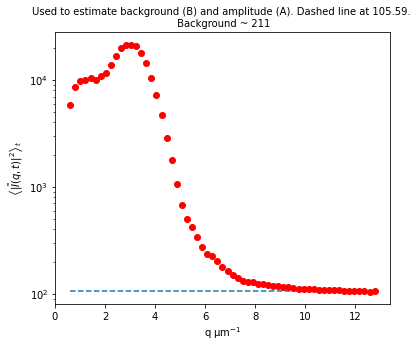
Note: There are a few optional arguments we can pass to calculate_DDM_matrix. There is an optional argument quiet (True or False, False by default). Then we have some optional keyword arguments (all of which could also be specified in the YAML file). These are: overlap_method which sets the degree of overlap between image pairs when finding all image differences for a each lag time and is either 0, 1, 2, or 3 (with 2 being the default), background_method which
sets how to estimate the background parameter B and is either 0, 1, 2, 3, 4, or 5 (with 0 being the default), amplitude_method which sets how to estimate the amplitude parameter A and is either 0, 1, or 2 (with 1 being the default), and number_lag_times. If any of these three keyword arguments are set here, the value specified in the YAML file will be overwritten.
[5]:
#If a file is found that matches what, by default, the program will save the computed DDM matrix as,
#then you will be prompted as to whether or not you want to proceed with this calculation. If you
#do not, then enter 'n' and the program will read from the existing file to load the DDM dataset
#into memory. If you enter 'y', then the DDM matrix will be calculated.

ddm_calc.calculate_DDM_matrix()
The file C:/Users/rmcgorty/Documents/GitHub/PyDDM/Examples/images_nobin_40x_128x128_8bit_ddmmatrix.nc already exists. So perhaps the DDM matrix was calculated already?
Do you still want to calculate the DDM matrix? (y/n):
2025-06-11 18:17:43,267 - DDM Calculations - Running dt = 1...
2025-06-11 18:17:44,976 - DDM Calculations - Running dt = 5...
2025-06-11 18:17:45,969 - DDM Calculations - Running dt = 9...
2025-06-11 18:17:46,667 - DDM Calculations - Running dt = 16...
2025-06-11 18:17:47,159 - DDM Calculations - Running dt = 27...
2025-06-11 18:17:47,568 - DDM Calculations - Running dt = 47...
2025-06-11 18:17:47,907 - DDM Calculations - Running dt = 81...
2025-06-11 18:17:48,196 - DDM Calculations - Running dt = 138...
2025-06-11 18:17:48,408 - DDM Calculations - Running dt = 236...
2025-06-11 18:17:48,599 - DDM Calculations - Running dt = 402...
C:\Users\rmcgorty\Documents\GitHub\PyDDM\docs\source\../../PyDDM\ddm_calc.py:1167: RuntimeWarning: invalid value encountered in true_divide
  ravs[0] = h/histo_of_bins
C:\Users\rmcgorty\Documents\GitHub\PyDDM\docs\source\../../PyDDM\ddm_calc.py:1172: RuntimeWarning: invalid value encountered in true_divide
  ravs[i] = h/histo_of_bins
DDM matrix took 5.470902919769287 seconds to compute.
 Background estimate ± std is 113.01 ± 4.56
[5]:
<xarray.Dataset>
Dimensions: (lagtime: 40, q_y: 64, q_x: 64, q: 32, y: 64, x: 64,
frames: 40)
Coordinates:
* lagtime (lagtime) float64 0.02398 0.04796 0.07194 ... 12.59 14.39
framelag (frames) int32 1 2 3 4 5 6 7 ... 308 352 402 459 525 600
* q_y (q_y) float64 -6.491 -6.288 -6.085 ... 5.882 6.085 6.288
* q_x (q_x) float64 -6.491 -6.288 -6.085 ... 5.882 6.085 6.288
* q (q) float64 0.0 0.2028 0.4057 0.6085 ... 5.882 6.085 6.288
* y (y) int32 0 1 2 3 4 5 6 7 8 ... 55 56 57 58 59 60 61 62 63
* x (x) int32 0 1 2 3 4 5 6 7 8 ... 55 56 57 58 59 60 61 62 63
Dimensions without coordinates: frames
Data variables:
ddm_matrix_full (lagtime, q_y, q_x) float64 53.61 52.11 ... 25.11 44.82
ddm_matrix (lagtime, q) float64 nan 95.51 94.07 ... 134.0 135.0 100.7
first_image (y, x) float64 151.0 176.5 203.5 ... 234.5 197.8 199.0
alignment_factor (lagtime, q) float64 nan 6.123e-17 ... 0.04203 0.02394
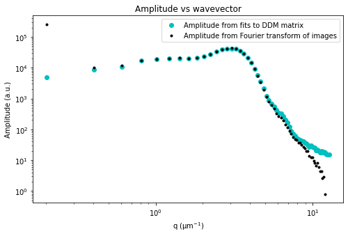
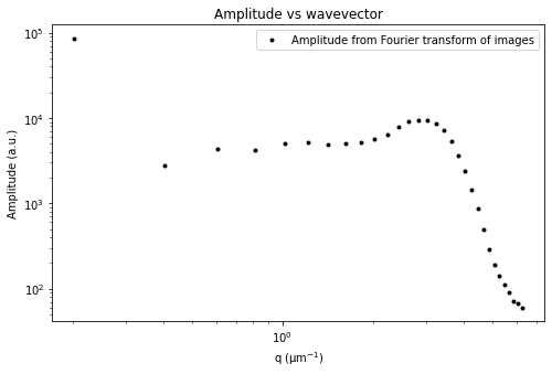
avg_image_ft (q) float64 nan 4.317e+04 1.392e+03 ... 59.15 56.79 53.58
ft_of_avg_image (q) float64 nan 4.267e+04 601.7 893.3 ... 2.234 2.34 2.257
num_pairs_per_dt (lagtime) int32 998 997 996 498 497 497 ... 7 6 5 4 3 2
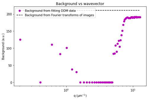
B float64 113.0
B_std float64 4.558
Amplitude (q) float64 nan 8.623e+04 2.671e+03 ... 0.5622 -5.843
ISF (lagtime, q) float64 nan 1.0 1.007 ... -2.978 -38.2 -1.113
Attributes: (12/26)
units: Intensity
lagtime: sec
q: μm$^{-1}$
x: pixels
y: pixels
info: ddm_matrix is the averages of FFT difference ima...
... ...
split_into_4_rois: False
use_windowing_function: False
binning: True
bin_size: 2
central_angle: None
angle_range: None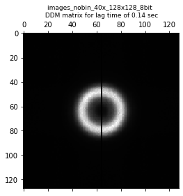
Initiazing DDM_Fit class and fitting our data to a model#
Next, we initialize the DDM_Fit class which will help us fit the calculated DDM matrix to a model of our choosing.
When the DDM_Fit class is initialized, it will display a table of the parameters, with the initial guesses and bounds, that were in the parameters of the yaml file. It will also indicate if, for the chosen model, initial guesses for parameters are missing.
Note: The intial guesses and bounds for the parameters are given in the yaml file. But you may realize that you need to adjust the bounds. You could change the yaml file and reload it. But you can also change the initial guesses and bounds for the parameters as shown in this code snippet:
ddm_fit.set_parameter_initial_guess('Tau', 0.5)
ddm_fit.set_parameter_bounds('Tau', [0.001, 1000])
Also, note that to initialize the DDM_Fit class, we need to pass it the YAML file which contains the metadata and parameters. Below, we use the fact that the path to the YAML file is stored in the variable ddm_calc.data_yaml. But we could also use the path to the YAML file just like we did when initializing the DDM_Analysis class. That is, this would work as well:
ddm_fit = ddm.DDM_Fit("../../Examples/example_data_silica_beads.yml")
[6]:
ddm_fit = ddm.DDM_Fit(ddm_calc.data_yaml)
| Initial guess | Minimum | Maximum | |
|---|---|---|---|
| Amplitude | 100.0 | 1.000 | 1000000.0 |
| Tau | 1.0 | 0.001 | 10.0 |
| Background | 25000.0 | 0.000 | 10000000.0 |
| StretchingExp | 1.0 | 0.500 | 1.1 |
Loading file C:/Users/rmcgorty/Documents/GitHub/PyDDM/Examples/images_nobin_40x_128x128_8bit_ddmmatrix.nc ...
Below, the fit is performed and saved into an xarray Dataset. We also have a table of the parameters for each q. Since this table may be long (especially if you have a large image size), you might want to not display it. If that’s the case, then run this command with the display_table parmeter set to False, i.e.:
fit01 = ddm_fit.fit(name_fit = 'fit01', display_table=False)
[7]:
#Note that the method `fit` has many optional parameters, but here we
# allow those optional parameter to take their default values

fit01 = ddm_fit.fit(name_fit = 'fit01')
In function 'get_tau_vs_q_fit', using new tau...
Fit is saved in fittings dictionary with key 'fit01'.
| q | Amplitude | Tau | Background | StretchingExp | |
|---|---|---|---|---|---|
| 0 | 0.000000 | 100.000000 | 1.000000 | 25000.000000 | 1.000000 |
| 1 | 0.202840 | 2221.053486 | 10.000000 | 105.857478 | 0.696463 |
| 2 | 0.405681 | 3006.600450 | 10.000000 | 8.836142 | 0.572435 |
| 3 | 0.608521 | 3718.728783 | 4.503455 | 0.000000 | 0.687558 |
| 4 | 0.811362 | 5092.262467 | 3.367577 | 0.000000 | 0.758814 |
| 5 | 1.014202 | 5298.076962 | 1.495877 | 0.000000 | 0.875560 |
| 6 | 1.217043 | 5017.826391 | 0.923533 | 0.000000 | 0.919762 |
| 7 | 1.419883 | 5018.286724 | 0.707998 | 0.000000 | 0.933032 |
| 8 | 1.622723 | 4804.352014 | 0.486938 | 0.000000 | 0.973702 |
| 9 | 1.825564 | 5181.793843 | 0.446446 | 0.000000 | 0.965262 |
| 10 | 2.028404 | 5611.243988 | 0.371388 | 0.000000 | 0.979897 |
| 11 | 2.231245 | 6403.155522 | 0.308168 | 0.000000 | 0.996226 |
| 12 | 2.434085 | 7812.097726 | 0.273778 | 0.000000 | 1.024677 |
| 13 | 2.636926 | 8842.276777 | 0.231335 | 0.000000 | 1.049213 |
| 14 | 2.839766 | 9033.580795 | 0.205506 | 0.000000 | 1.034606 |
| 15 | 3.042607 | 9228.078528 | 0.190861 | 0.000000 | 1.036096 |
| 16 | 3.245447 | 8215.724811 | 0.166399 | 0.000000 | 1.037051 |
| 17 | 3.448287 | 7064.034828 | 0.153635 | 0.000000 | 1.040212 |
| 18 | 3.651128 | 5159.959987 | 0.139709 | 0.000000 | 1.032205 |
| 19 | 3.853968 | 3564.060652 | 0.127278 | 0.000000 | 1.037030 |
| 20 | 4.056809 | 2320.133466 | 0.118597 | 0.000000 | 1.026376 |
| 21 | 4.259649 | 1422.696297 | 0.111623 | 0.000000 | 0.998286 |
| 22 | 4.462490 | 866.841353 | 0.102422 | 0.000000 | 0.964719 |
| 23 | 4.665330 | 514.012003 | 0.098157 | 6.102412 | 0.915522 |
| 24 | 4.868170 | 301.203055 | 0.094404 | 18.732899 | 0.890644 |
| 25 | 5.071011 | 194.349793 | 0.101695 | 31.757336 | 0.885361 |
| 26 | 5.273851 | 152.163959 | 0.094730 | 28.431701 | 0.801239 |
| 27 | 5.476692 | 118.809414 | 0.095692 | 32.667078 | 0.789463 |
| 28 | 5.679532 | 96.618516 | 0.098254 | 34.735010 | 0.754149 |
| 29 | 5.882373 | 77.994077 | 0.109526 | 38.194460 | 0.746305 |
| 30 | 6.085213 | 73.573291 | 0.109010 | 37.473100 | 0.710879 |
| 31 | 6.288053 | 66.603954 | 0.101589 | 36.948208 | 0.686781 |
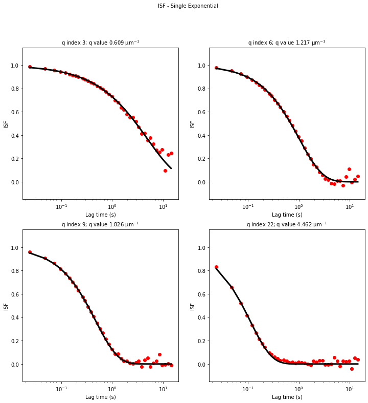
Inspecting the outcome of the fit#
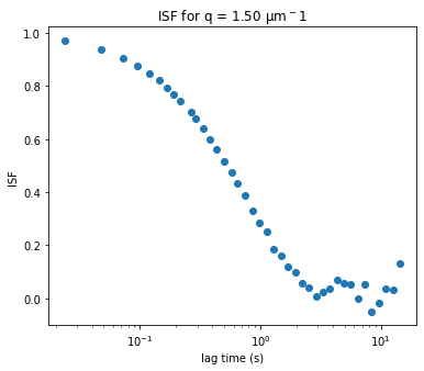
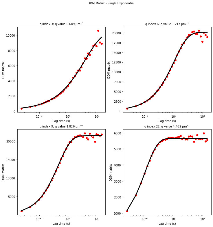
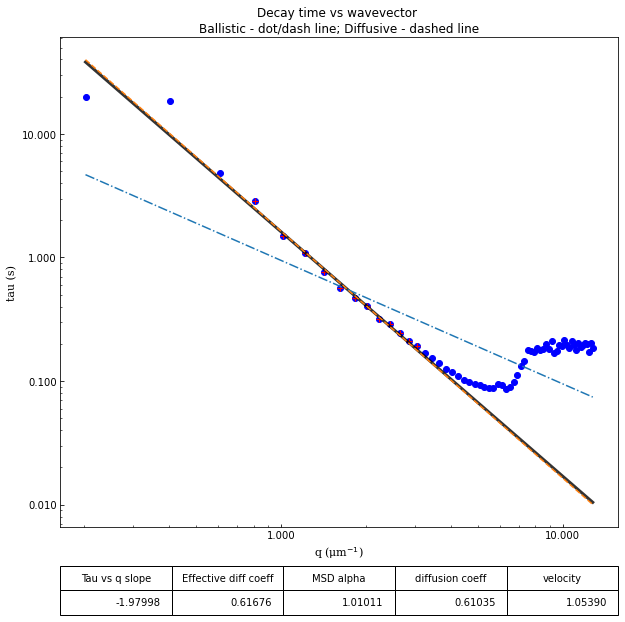
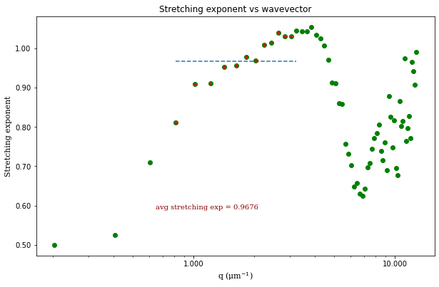
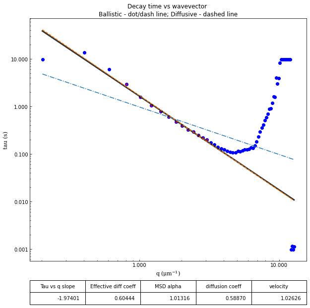
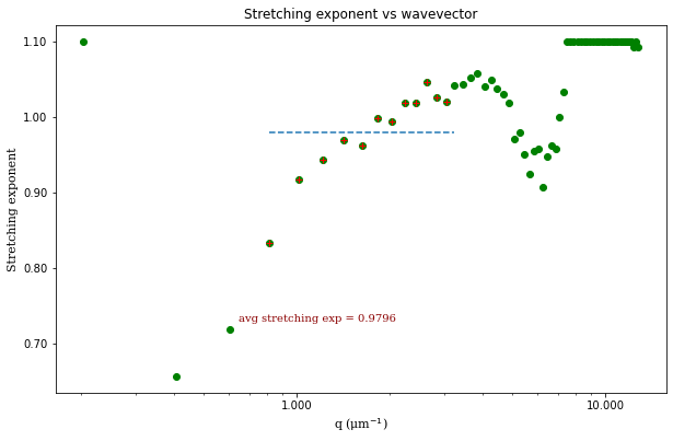
We can now take a look at the best fit parameters determined by the fitting code. We can generate a set of plots and have the output saved as PDF with the function fit_report. This takes a few arguments, including:
the result of the fit in an xarray Dataset (here
fit01)q_indices: the DDM matrix or the ISF (whichever was used in the fitting) will be plotted at these \(q\)-values specified by their index in the array of \(q\)-valuesforced_qs: range of \(q\)-values (specified, again, by the index) for which to extract power law relationship between the decay time \(\tau\) and \(q\)
[8]:
ddm.fit_report(fit01, q_indices=[3,6,9,22], forced_qs=[4,16], use_new_tau=True, show=True)
In function 'get_tau_vs_q_fit', using new tau...
In hf.plot_one_tau_vs_q function, using new tau...
[8]:
<xarray.Dataset>
Dimensions:          (parameter: 4, q: 32, lagtime: 40)
Coordinates:
  * parameter        (parameter) <U13 'Amplitude' 'Tau' ... 'StretchingExp'
  * q                (q) float64 0.0 0.2028 0.4057 0.6085 ... 5.882 6.085 6.288
  * lagtime          (lagtime) float64 0.02398 0.04796 0.07194 ... 12.59 14.39
Data variables:
    parameters       (parameter, q) float64 100.0 2.221e+03 ... 0.7109 0.6868
    theory           (lagtime, q) float64 2.5e+04 138.9 102.5 ... 111.0 103.6
    isf_data         (lagtime, q) float64 nan 1.0 1.007 ... -2.978 -38.2 -1.113
    ddm_matrix_data  (lagtime, q) float64 nan 95.51 94.07 ... 134.0 135.0 100.7
    A                (q) float64 nan 8.623e+04 2.671e+03 ... 5.281 0.5622 -5.843
    B                float64 113.0
Attributes: (12/18)
    model:                          DDM Matrix - Single Exponential
    data_to_use:                    DDM Matrix
    initial_params_dict:            ["{'n': 0, 'value': 100.0, 'limits': [1.0...
    effective_diffusion_coeff:      0.6953227734274584
    tau_vs_q_slope:                 [-1.89509843]
    msd_alpha:                      [1.05535415]
    ...                             ...
    DataDirectory:                  C:/Users/rmcgorty/Documents/GitHub/PyDDM/...
    FileName:                       images_nobin_40x_128x128_8bit.tif
    pixel_size:                     0.242
    frame_rate:                     41.7
    BackgroundMethod:               0
    OverlapMethod:                  2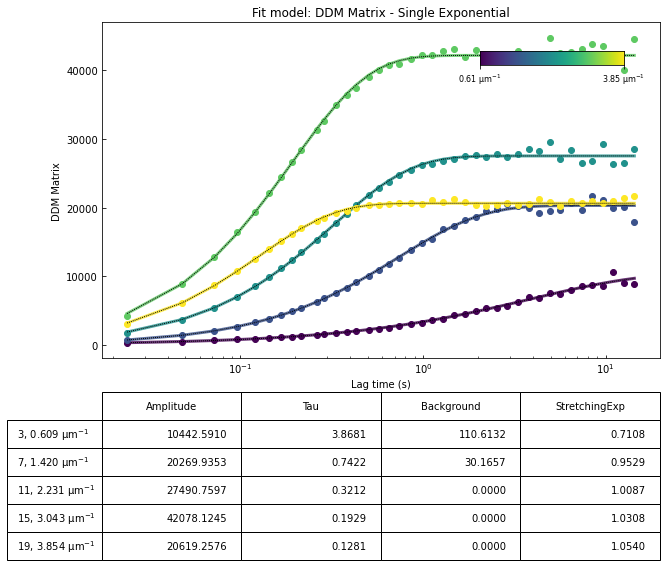
Trying a different mathematical model#
Above, we fit the DDM matrix to a model where the intermediate scattering function (ISF or \(f(q,\Delta t)\)) is an exponential. That is, we fit our data to:
where \(A\) is the amplitude, \(B\) is the background, \(\tau\) is the decay time, and \(s\) is the stretching exponent.
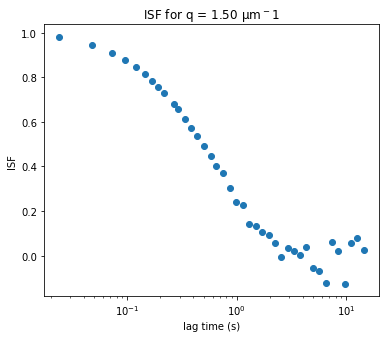
An alternative is to use other information to determine \(A(q)\) and \(B\) and then fit only the ISF. We will try this below.
[9]:
ddm_fit.reload_fit_model_by_name("ISF - Single Exponential")
| Initial guess | Minimum | Maximum | |
|---|---|---|---|
| Tau | 1.0 | 0.001 | 10.0 |
| StretchingExp | 1.0 | 0.500 | 1.1 |
[10]:
fit02 = ddm_fit.fit(name_fit = 'fit02', display_table=False)
In function 'get_tau_vs_q_fit', using new tau...
Fit is saved in fittings dictionary with key 'fit02'.
[11]:
ddm.fit_report(fit02, q_indices=[3,6,9,22], forced_qs=[4,16], use_new_tau=True, show=True)
In function 'get_tau_vs_q_fit', using new tau...
In hf.plot_one_tau_vs_q function, using new tau...
[11]:
<xarray.Dataset>
Dimensions:          (parameter: 2, q: 32, lagtime: 40)
Coordinates:
  * parameter        (parameter) <U13 'Tau' 'StretchingExp'
  * q                (q) float64 0.0 0.2028 0.4057 0.6085 ... 5.882 6.085 6.288
  * lagtime          (lagtime) float64 0.02398 0.04796 0.07194 ... 12.59 14.39
Data variables:
    parameters       (parameter, q) float64 1.0 10.0 7.188 5.93 ... 1.1 1.1 1.08
    theory           (lagtime, q) float64 0.9763 0.9987 0.984 ... 0.2249 0.0
    isf_data         (lagtime, q) float64 nan 1.0 1.007 ... -2.978 -38.2 -1.113
    ddm_matrix_data  (lagtime, q) float64 nan 95.51 94.07 ... 134.0 135.0 100.7
    A                (q) float64 nan 8.623e+04 2.671e+03 ... 5.281 0.5622 -5.843
    B                float64 113.0
Attributes: (12/18)
    model:                          ISF - Single Exponential
    data_to_use:                    ISF
    initial_params_dict:            ["{'n': 0, 'value': 1.0, 'limits': [0.001...
    effective_diffusion_coeff:      0.7036941102436204
    tau_vs_q_slope:                 [-1.86108913]
    msd_alpha:                      [1.07463956]
    ...                             ...
    DataDirectory:                  C:/Users/rmcgorty/Documents/GitHub/PyDDM/...
    FileName:                       images_nobin_40x_128x128_8bit.tif
    pixel_size:                     0.242
    frame_rate:                     41.7
    BackgroundMethod:               0
    OverlapMethod:                  2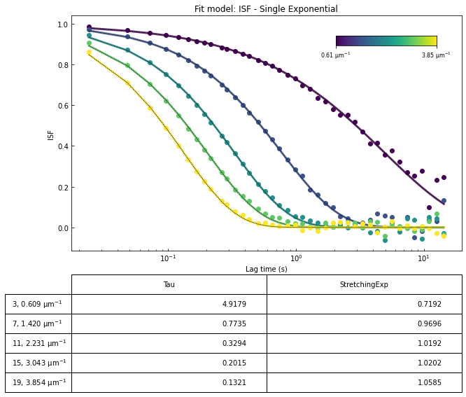
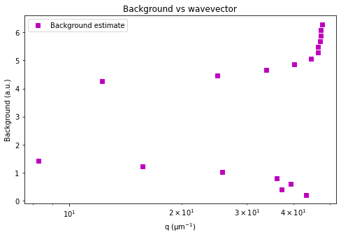
Switching method for calculating background#
[12]:
ddm_fit.ddm_dataset = ddm.recalculate_ISF_with_new_background(ddm_fit.ddm_dataset, background_method=5)
[13]:
ddm_fit.reload_fit_model_by_name("ISF - Single Exponential")
| Initial guess | Minimum | Maximum | |
|---|---|---|---|
| Tau | 1.0 | 0.001 | 10.0 |
| StretchingExp | 1.0 | 0.500 | 1.1 |
[14]:
fit03 = ddm_fit.fit(name_fit = 'fit03', display_table=False)
In function 'get_tau_vs_q_fit', using new tau...
Fit is saved in fittings dictionary with key 'fit03'.
[15]:
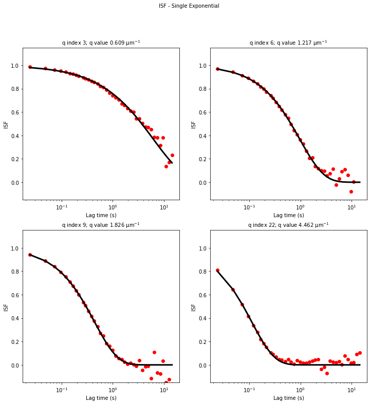
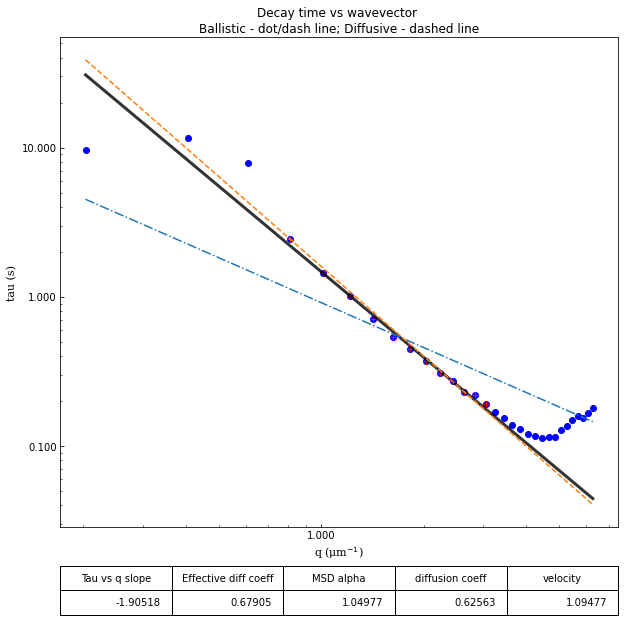
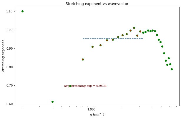
ddm.fit_report(fit03, q_indices=[3,6,9,22], forced_qs=[4,16], use_new_tau=True, show=True)
In function 'get_tau_vs_q_fit', using new tau...
In hf.plot_one_tau_vs_q function, using new tau...
[15]:
<xarray.Dataset>
Dimensions:          (parameter: 2, q: 32, lagtime: 40)
Coordinates:
  * parameter        (parameter) <U13 'Tau' 'StretchingExp'
  * q                (q) float64 0.0 0.2028 0.4057 0.6085 ... 5.882 6.085 6.288
  * lagtime          (lagtime) float64 0.02398 0.04796 0.07194 ... 12.59 14.39
Data variables:
    parameters       (parameter, q) float64 1.0 10.0 7.946 ... 0.8157 0.788
    theory           (lagtime, q) float64 0.9763 0.9987 ... 8.265e-19 4.399e-16
    isf_data         (lagtime, q) float64 nan 0.9994 0.9793 ... -0.3241 0.1094
    ddm_matrix_data  (lagtime, q) float64 nan 95.51 94.07 ... 134.0 135.0 100.7
    A                (q) float64 nan 8.63e+04 2.747e+03 ... 70.99 66.27 59.49
    B                (q) float64 0.0 43.19 37.14 39.34 ... 47.17 47.3 47.3 47.68
Attributes: (12/18)
    model:                          ISF - Single Exponential
    data_to_use:                    ISF
    initial_params_dict:            ["{'n': 0, 'value': 1.0, 'limits': [0.001...
    effective_diffusion_coeff:      0.6790467087346614
    tau_vs_q_slope:                 [-1.90518355]
    msd_alpha:                      [1.04976762]
    ...                             ...
    DataDirectory:                  C:/Users/rmcgorty/Documents/GitHub/PyDDM/...
    FileName:                       images_nobin_40x_128x128_8bit.tif
    pixel_size:                     0.242
    frame_rate:                     41.7
    BackgroundMethod:               5
    OverlapMethod:                  2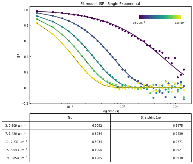
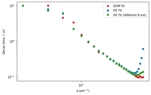
Comparing fit methods#
[16]:
fig, ax = plt.subplots(figsize=(8,8/1.618))

q_lo, q_hi = 1,28
ax.loglog(fit01.q[q_lo:q_hi], fit01.parameters.loc['Tau'][q_lo:q_hi], 'o', c='tab:red', label="DDM Fit")
ax.loglog(fit02.q[q_lo:q_hi], fit02.parameters.loc['Tau'][q_lo:q_hi], 'o', c='tab:blue', label="ISF Fit")
ax.loglog(fit03.q[q_lo:q_hi], fit03.parameters.loc['Tau'][q_lo:q_hi], 'o', c='tab:green', label="ISF Fit (different B est)")

plt.legend(loc=0)

ax.set_xlabel("$q$ ($\mu$m$^{-1}$)")
ax.set_ylabel("Decay time, $\\tau$ (s)")
[16]:
Text(0, 0.5, 'Decay time, $\\tau$ (s)')
Interactive with matplotlib#
Using the Browse_DDM_Fits class as shown below, one can interactively inspect the fits (to either the DDM matrix or the ISF) by selecting the appropriate point on the \(\tau\) vs \(q\) plot or by pressing ‘N’ or ‘P’ for next or previous.
[17]:
%matplotlib notebook
fig, (ax, ax2) = plt.subplots(2, 1, figsize=(10,10/1.618))
browser = ddm.Browse_DDM_Fits(fig, ax, ax2, fit02)

fig.canvas.mpl_connect('pick_event', browser.on_pick)
fig.canvas.mpl_connect('key_press_event', browser.on_press)

ax.set_title('Decay time vs wavevector')
ax.set_xlabel("q")
ax.set_ylabel("tau (s)")

Click on a point in the tau vs q plot to see a fit.
Or press 'N' or 'P' to display next or previous fit.
[17]:
Text(0, 0.5, 'tau (s)')
[ ]:
Saving the results#
We have a few options for saving the results of the fit. We can save the information contained in the xarray Dataset fit01 as an Excel file. Or we can save it as a netCDF file using the xarray function `to_netcdf <https://xarray.pydata.org/en/stable/generated/xarray.Dataset.to_netcdf.html>`__. If we have the fit results as a netCDF file, then we can reload it easily with teh xarray function `open_dataset <https://xarray.pydata.org/en/stable/generated/xarray.open_dataset.html>`__.
[13]:
ddm.save_fit_results_to_excel(fit01)
[14]:
fit01.to_netcdf("fit_of_ddmmatrix.nc")